3. Sorting #

Created Sat May 18, 2024 at 11:14 AM

#sorting

Why sorting #

Sorting is an important subroutine in many algorithms. Even big data stuff like MapReduce keeps stuff sorted just because it makes operations faster.

API #

2-Algorithms

Solving use #

• Searching - Binary search becomes possible after sorting.
• Closest-pair: Given n number find closest pair. Sort and traverse (and count min difference).
• Element uniqueness - are there any duplicates. Sort and traverse (for all unique). Can check if given element us unique too - using low and upper bound.
• Find the mode (most occurring) - sort and traverse (linear). If already sorted, use low and upper bound (logn).
• Selection (kth largest/smallest) - assuming duplicate answer is fine, this is just the k th element. Median is also simple thing way (k/2th element).
• Convex hulls - Skiena 111.

Hashing vs Sorting #

Sometimes, Hashing can solve faster than sorting. Example - uniqueness check, counting is better with hashing.

Other-times, hashing may not be appropriate - convex hull ago.

Practical use #

TBD

Algorithms #

Sure, here’s a list of common sorting algorithms, including both those with O(N^2) time complexity and more efficient ones:

Comparative #

1. Bubble Sort (O(N^2)): aka bubble to the right while swapping, compares adjacent elements and swaps them if they are in the wrong order, repeating this process until the list is sorted. Also keeps a is_sorted flag in each loop for early return. Complexity same on linked list.
2. Insertion Sort (O(N^2)) insert at the correct position, forms sorted array at the end: Builds the final sorted list one item at a time by repeatedly taking elements from the input list and inserting them into their correct positions in the sorted list. Only online algorithm (since its general insert, can accommodate for new data). We can use binary search to find the spot, but shifting would still cause squared complexity.
3. Selection Sort (O(N^2)): min select and swap, form sorted array. Divides the input list into a sorted sublist and an unsorted sublist, repeatedly finding the smallest (or largest) element from the unsorted sublist and moving it to the end of the sorted sublist.
4. Merge Sort (O(N log N), O(N) space): Divides the input list into two halves, recursively sorts each half, and then merges the sorted halves to produce the final sorted list. It’s a divide-and-conquer algorithm and typically faster than the quadratic-time sorting algorithms for large datasets.
5. Quick Sort (O(N log N) average, O(N^2) worst-case, O(N) space): Randomly selects a “pivot” element from the list and partitions the other elements into two sublists according to whether they are less than or greater than the pivot. It then recursively sorts the sublists.
6. Heap Sort (O(N log N) time, O(1) space) - “an implementation of selection sort using the right data structure.”: Builds a binary heap from the input list and repeatedly extracts the maximum (for a max heap) element from the heap and rebuilds the heap until the list is sorted. It’s not stable but has a guaranteed worst-case time complexity. O(1) space.

Non-comparative #

7. Counting Sort (O(N + K) time, O(k) space): Works well when the range of input elements is small. It counts the number of occurrences of each element and uses this information to place each element into its correct position in the output sequence.
8. Bucket Sort (O(N + K) time, O(N+K) space): Distributes elements into a number of “buckets” and then sorts each bucket individually, typically using another sorting algorithm like insertion sort or quick-sort. It’s efficient when the input is uniformly distributed over a range.
9. Radix Sort (O(NK) time, O(N+K) space): Sorts elements by processing individual digits of the numbers. It starts by sorting elements based on their least significant digit and progressively moves towards the most significant digit. Radix sort can achieve linear time complexity for integer sorting when the number of digits (K) is considered a constant.

These algorithms offer different trade-offs in terms of time complexity, space complexity, and suitability for different types of data. Radix sort, counting sort, and bucket sort, in particular, are often used in scenarios where the input data has specific characteristics that make these algorithms more efficient than traditional comparison-based sorting algorithms like quick-sort and merge sort.

These are some of the common sorting algorithms, each with its own characteristics and best use cases depending on factors like the size of the dataset and stability requirements.

Note:

• Sort for linked lists:
  1. Merge sort. nlogn time, O(1) space (since in place merge is possible).
  2. All squared sorts - insertion sort especially (overhead of shifting by 1 is removed)
  3. Quick sort - bad, since partitioning requires random access.
• Comparison of squared sorts:
  1. Bubble sort - for educational purpose only. Too many swaps (bad for device lifetime). Not used in practice.
  2. Selection sort - least swaps (good for device).
  3. Insertion sort - online. Good for partially sorted data.

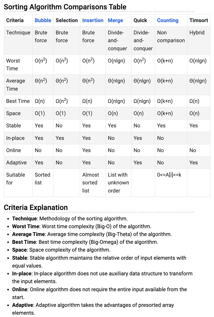
Comparison of sorting algorithms #

Note:

• Quick sort is not adaptive.